
The boundary layer is the thin region of fluid immediately next to a solid surface where velocity rises from zero at the wall (the no-slip condition) to roughly 99% of the free-stream velocity. Within this layer, viscous (friction) forces dominate; outside it, the flow behaves as if it were inviscid. The concept, introduced by Ludwig Prandtl in 1904, explains skin-friction drag, heat transfer and flow separation, and is fundamental to aerodynamics, pipe flow and heat-exchanger design.
Equipment mentioned in this guide
Review the product information, specifications and model before requesting a quotation.
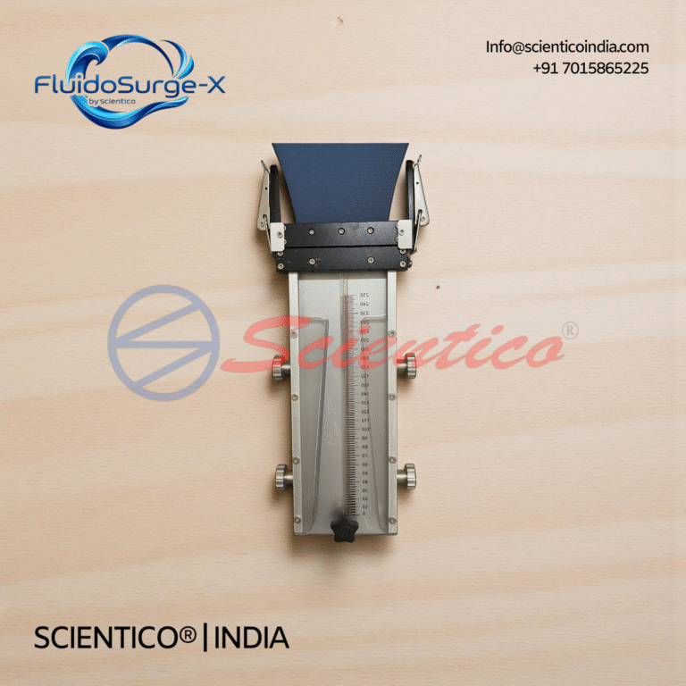
Boundary Layers Module | FluidoSurge-X 356
The Boundary Layers Module FluidoSurge-X 356 is a laboratory accessory designed for experimental investigation of boundary layer development over a flat plate. Manufactured by SCIENTICO, the unit enables detailed study of laminar and turbulent boundary layers and the influence of surface roughness. It is intended for use with the compatible aerodynamics trainer in fluid mechanics laboratories.
View product detailsWhy does a boundary layer form?
A real (viscous) fluid sticks to a solid surface. At the wall, fluid velocity equals the surface velocity (zero for a stationary plate), this is the no-slip condition. Each layer of fluid drags the next through viscosity, so velocity increases gradually with distance from the wall until it matches the free stream. That velocity-gradient region is the boundary layer. It governs:
- Skin-friction drag, the wall shear stress acting on the surface.
- Heat and mass transfer, the thermal/concentration boundary layer controls heat-exchanger and reactor performance.
- Flow separation, which sets pressure (form) drag, stall and wake size.
How is boundary-layer thickness defined?
Several thickness measures are used, all with units of length (m or mm):
- Boundary-layer thickness (δ), the distance from the wall at which u = 0.99 U∞, where U∞ is the free-stream velocity.
- Displacement thickness (δ*), the distance the surface would notionally move outward to give the same mass-flow deficit: δ* = ∫0δ(1 − u/U∞) dy.
- Momentum thickness (θ), represents the momentum-flux deficit: θ = ∫0δ(u/U∞)(1 − u/U∞) dy.
For laminar flow over a flat plate, the Blasius solution gives δ ≈ 5.0·x / √Rex, where x is the distance from the leading edge and Rex = U∞ x / ν is the local Reynolds number (ν = kinematic viscosity, m²/s). Because δ grows with √x, the layer thickens downstream.
What is the difference between laminar and turbulent boundary layers?
The flow regime is set by the Reynolds number. On a smooth flat plate, transition typically begins near Rex ≈ 5 × 10⁵ (the exact value depends on surface roughness, free-stream turbulence and pressure gradient).
| Property | Laminar boundary layer | Turbulent boundary layer |
|---|---|---|
| Flow structure | Smooth, ordered, parallel layers | Chaotic, with eddies and mixing |
| Typical Rex (flat plate) | Below ~5 × 10⁵ | Above ~5 × 10⁵ |
| Velocity profile | Nearly parabolic, gentle wall slope | Fuller, steep gradient at wall |
| Thickness growth | δ ∝ x0.5 | δ ∝ x0.8 (grows faster) |
| Wall shear / skin friction | Lower | Higher |
| Mixing & heat transfer | Low | High |
| Resistance to separation | Separates more easily | Stays attached longer |
A turbulent layer carries higher-momentum fluid close to the wall, so it has more skin-friction drag but resists separation better, which is why golf balls are dimpled and many aerofoils trip the flow turbulent.
What is boundary-layer separation?
Separation occurs when the flow can no longer follow the surface and lifts away, leaving a recirculating wake. It is caused by an adverse pressure gradient (pressure rising in the flow direction, dp/dx > 0), which decelerates the slow near-wall fluid until it reverses. At the separation point the wall shear stress falls to zero (∂u/∂y = 0 at the wall).
Consequences and controls:
- Increased pressure (form) drag and energy loss.
- Loss of lift / stall on aerofoils and turbine blades.
- Mitigation: streamlining, tripping to turbulence, vortex generators, suction or blowing, and avoiding sharp area changes.
Where does the boundary layer matter in engineering?
- Aerodynamics, wings, fuselages, drag and stall prediction.
- Internal/pipe flow, entry length, friction factor and pump sizing.
- Heat exchangers, the thermal boundary layer limits the convective heat-transfer coefficient.
- Turbomachinery, blade losses and efficiency.
- Civil/wind engineering, the atmospheric boundary layer over terrain and structures.
How do you select boundary-layer lab equipment?
For engineering colleges and universities building a fluid mechanics lab, evaluate teaching apparatus against these criteria:
- Measurable range: Reynolds numbers spanning laminar, transition and turbulent regimes so students see all three.
- Instrumentation: a traversing Pitot tube or hot-wire probe with a micrometer/digital traverse to map velocity profiles and compute δ, δ* and θ.
- Flow visualization: smoke, dye or tuft methods to show transition and separation clearly.
- Test section: flat plate, aerofoil or curved-wall models for separation studies; interchangeable models add value.
- Construction: corrosion-resistant frames, transparent working sections (acrylic/glass) and stable, calibrated manometry or transducers.
- Safety & standards: guarded fans/pumps, stable mountings, clear manuals and compliance documentation.
- Curriculum fit: alignment with your syllabus, repeatable results and supporting lab manuals.
- Lifecycle: spares availability, warranty, installation/commissioning and after-sales support, critical for export buyers.
What to ask a supplier (procurement checklist)
- What velocity/Reynolds-number range does the apparatus cover, and is transition demonstrable?
- What measurement resolution does the traverse and manometer/transducer provide?
- Are calibration certificates and a detailed lab manual with sample readings included?
- What quality certifications do you hold (e.g., ISO 9001:2015, CE)?
- Do you supply spare parts, and what is the warranty and lead time?
- Can you provide installation, commissioning and operator training?
- For export: do you quote CIF, and what are packing, documentation and delivery timelines?
- Are you registered on procurement portals (e.g., GeM) for Indian institutions?
How is the boundary layer shown and measured in a teaching lab?
In a typical fluid mechanics lab, a flat plate or aerofoil is mounted in a wind tunnel or water channel. Students traverse a Pitot-static or hot-wire probe across the layer to record velocity u versus distance y, then plot the velocity profile and locate δ at u = 0.99 U∞. Numerical integration of the profile yields displacement thickness δ* and momentum thickness θ, while smoke or dye visualization reveals transition and the separation point under an adverse pressure gradient. Comparing measured δ against the Blasius estimate δ ≈ 5.0·x/√Rex reinforces the theory.
Scientico India manufactures and exports ISO 9001:2015 and model-specific fluid mechanics and engineering lab equipment from Ambala, India, supporting colleges and universities across 30+ countries. Explore our Fluid Mechanics Lab Equipment range for boundary-layer, wind-tunnel and flow-measurement teaching apparatus.
Frequently Asked Questions
What is the boundary layer in simple terms?
It is the thin layer of fluid right next to a solid surface where velocity changes from zero at the wall (no-slip condition) up to about 99% of the free-stream velocity. Friction (viscous) forces dominate inside this layer.
What is the difference between laminar and turbulent boundary layers?
A laminar boundary layer has smooth, ordered flow with lower skin friction but separates easily. A turbulent boundary layer has chaotic mixing, higher skin friction and steeper near-wall velocity, but resists separation better. On a flat plate, transition typically begins near a Reynolds number of about 5 x 10^5.
What causes boundary-layer separation?
Separation is caused by an adverse pressure gradient (pressure rising in the flow direction). It decelerates the slow near-wall fluid until it reverses and lifts off the surface, where wall shear stress drops to zero. This increases pressure drag and can cause stall.
How is boundary-layer thickness calculated for a flat plate?
For laminar flow, the Blasius solution gives delta approximately 5.0*x / sqrt(Re_x), where x is distance from the leading edge and Re_x = U_inf * x / nu is the local Reynolds number. Thickness grows with the square root of x.
How is the boundary layer measured in a teaching lab?
Students traverse a Pitot-static or hot-wire probe across the layer to record velocity versus distance, plot the velocity profile, and locate delta where u equals 0.99 of the free-stream velocity. Integrating the profile gives displacement and momentum thickness, and smoke or dye visualization shows transition and separation.
One honest ask
We don't gate anything on this site. You just read the whole thing free. If it was useful, leave your email and two things happen: we send you this page as a plain-text block you can paste into a tender file or an internal email, and we notify you the next time we publish a buyer tool like this one. Nothing else. No drip sequence, no sales calls booked without asking.