
This engineering lab glossary defines the core terms behind undergraduate engineering experiments, each with its formula, variables, units, and the laboratory apparatus that demonstrates it. It covers four disciplines: fluid mechanics, heat transfer & thermodynamics, strength of materials, and theory of machines. Definitions are written to be precise and self-contained, so you can use this as a quick reference for lab vivas, report writing, or specifying equipment for a new lab.
Equipment mentioned in this guide
Review the product information, specifications and model before requesting a quotation.
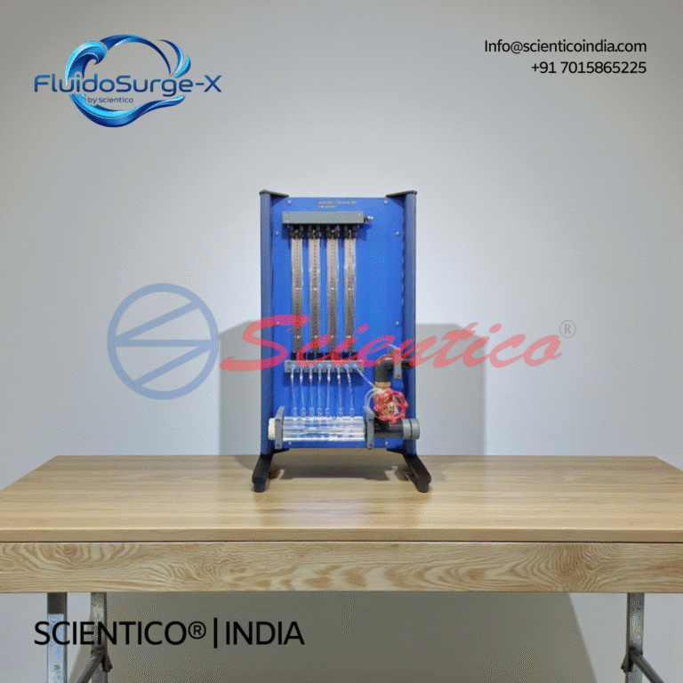
Bernoulli’s Theorem Apparatus | FluidoSurge-X 120
The Bernoulli's Theorem Apparatus FluidoSurge-X 120 is designed for experimental verification of Bernoulli’s principle in fluid mechanics laboratories. It enables detailed study of pressure, velocity, and energy variations along a converging and diverging duct. The apparatus uses a transparent Venturi test section with multiple pressure tapping points. It is intended for structured academic experiments and analytical comparison with theoretical flow behavior.
View product details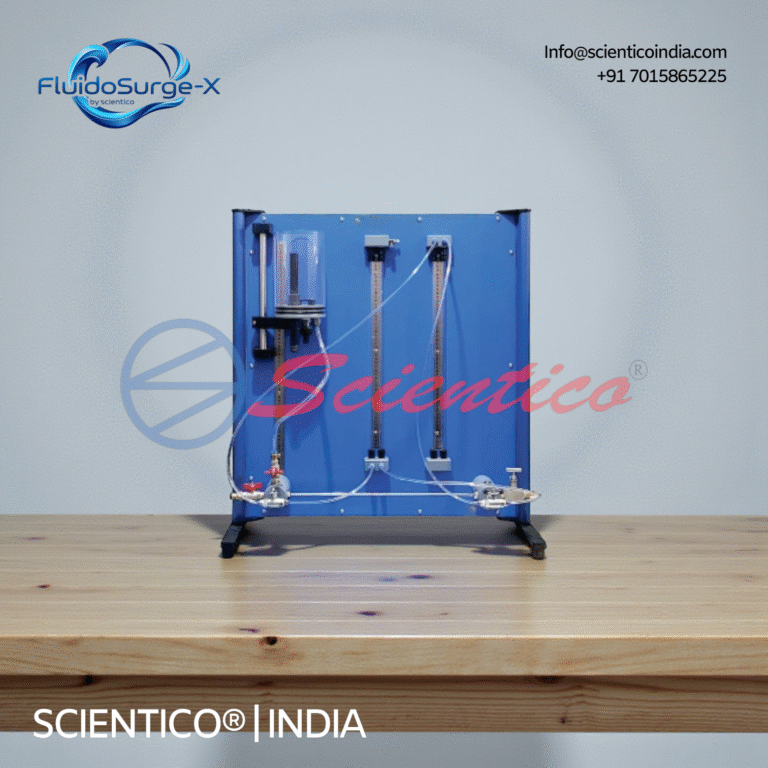
Pipe Friction Apparatus | FluidoSurge-X 168
The Pipe Friction Apparatus FluidoSurge-X 168 is designed for experimental determination of friction losses in pipe flow. It enables study of both laminar and turbulent flow regimes under controlled conditions. The apparatus allows measurement of head loss and determination of critical Reynolds number. It is suitable for fluid mechanics laboratory instruction and experimental analysis.
View product details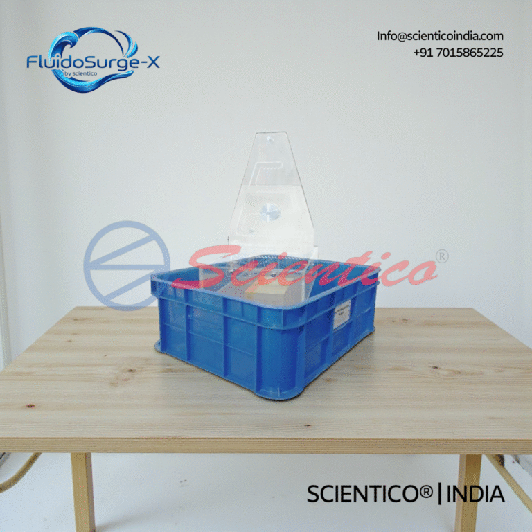
Metacentric Height Apparatus | FluidoSurgeX 108
The Metacentric Height Apparatus FluidoSurgeX 108 is designed for the experimental determination of the metacentric height of a floating body, a fundamental concept in naval architecture and fluid mechanics. The apparatus demonstrates the stability conditions of floating vessels and the relationship between the centre of buoyancy, centre of gravity, and metacentre.
View product details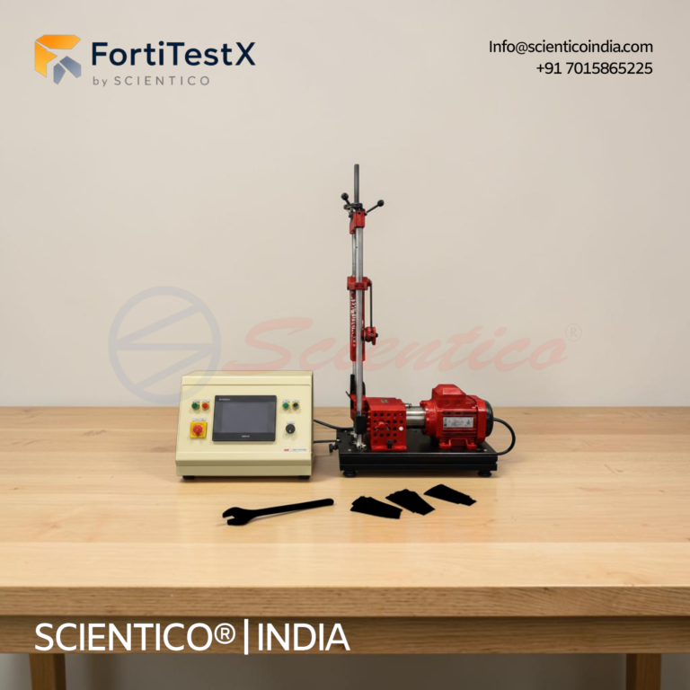
Fatigue Testing Machine | FortiTestX – 22
Fatigue Testing Machine FortiTestX 22 is a benchtop strength of materials lab equipment unit designed for fatigue strength testing of cylindrical metal specimens under cyclic bending load using a rotating cantilever configuration. This Fatigue Testing Machine clamps a revolving metal test bar at one end, applies a controlled point force via a spring balance and moveable plain bearing, and subjects the specimen to a sinusoidal bending stress cycle until fracture, with automatic shutdown triggered by a stop switch integrated into the bearing. The FortiTestX 22 includes an 8-digit electronic load cycle and revolutions counter with contactless inductive speed sensor, making it a complete fatigue testing machine strength of materials lab equipment unit for undergraduate materials testing and failure analysis programmes.
View product detailsFluid mechanics
Bernoulli’s equation
Bernoulli’s equation states that for steady, incompressible, frictionless flow along a streamline, the sum of pressure head, velocity head, and elevation head is constant: P/ρg + v²/2g + z = constant, where P is pressure (Pa), ρ is density (kg/m³), v is velocity (m/s), g is 9.81 m/s², and z is elevation (m). It expresses conservation of energy in a moving fluid. Demonstrated on a Bernoulli’s theorem apparatus.
Reynolds number (Re)
The Reynolds number is a dimensionless ratio of inertial to viscous forces that predicts whether flow is laminar or turbulent: Re = ρvD/μ = vD/ν, where D is the characteristic length/diameter (m), μ is dynamic viscosity (Pa·s) and ν is kinematic viscosity (m²/s). In pipe flow, Re < 2000 is laminar and Re > 4000 is turbulent. Demonstrated on a Reynolds number apparatus.
Metacentric height (GM)
Metacentric height is the distance between a floating body’s centre of gravity (G) and its metacentre (M); it measures stability, a larger GM means greater stability. Experimentally, GM = (w·d)/(W·tanθ), where w is the movable load, d its shift, W the total weight, and θ the tilt angle. Demonstrated on a metacentric height apparatus.
Coefficient of discharge (Cd)
The coefficient of discharge is the ratio of actual to theoretical discharge through a flow device: Cd = Qactual / Qtheoretical. It accounts for friction and contraction losses and is typically 0.6–0.98 depending on the device. Measured using a flow-measurement apparatus (venturi, orifice, rotameter).
Darcy–Weisbach friction head loss
The Darcy–Weisbach equation gives major head loss due to friction in a pipe: hf = f·(L/D)·(v²/2g), where f is the Darcy friction factor, L is pipe length (m) and D is diameter (m). It is the standard way to size pumping heads. Demonstrated on a pipe friction apparatus.
Impact (momentum) of a jet
The force a fluid jet exerts on a surface follows from the momentum equation: for a jet striking a stationary flat plate normally, F = ρQv, where Q is the volumetric flow rate (m³/s) and v the jet velocity (m/s); for a curved vane deflecting the jet by angle θ, F = ρQv(1 + cos θ). Demonstrated on an impact of jet on vanes apparatus.
Froude number (Fr)
The Froude number is a dimensionless ratio of inertial to gravitational forces, used mainly in open-channel and free-surface flow: Fr = v/√(gL), where L is a characteristic length (m). Fr < 1 is subcritical flow, Fr = 1 is critical, and Fr > 1 is supercritical.
Cavitation
Cavitation is the formation and rapid collapse of vapour bubbles in a liquid when the local static pressure falls below the liquid’s vapour pressure. The collapsing bubbles produce shock waves that pit and erode pump impellers and turbine blades, so avoiding it governs the design of pumps and hydraulic turbines.
Heat transfer & thermodynamics
Thermal conductivity (Fourier’s law)
Thermal conductivity (k) is a material property quantifying its ability to conduct heat, governed by Fourier’s law: Q = −kA(dT/dx), where Q is heat rate (W), A is area (m²), and dT/dx is the temperature gradient (K/m); k has units W/m·K. Demonstrated on a heat conduction apparatus (linear & radial).
Log mean temperature difference (LMTD)
LMTD is the effective average temperature difference driving heat transfer in a heat exchanger: ΔTlm = (ΔT₁ − ΔT₂) / ln(ΔT₁/ΔT₂), where ΔT₁ and ΔT₂ are the terminal temperature differences. Heat duty is then Q = U·A·ΔTlm. Demonstrated on a double-pipe heat exchanger.
Convective heat transfer coefficient (h)
The convective heat transfer coefficient quantifies heat exchange between a surface and a moving fluid, defined by Newton’s law of cooling: Q = hA(Ts − T∞), where h has units W/m²·K, Ts is surface temperature and T∞ the fluid temperature. Demonstrated on a natural & forced convection apparatus.
Stefan–Boltzmann law
The Stefan–Boltzmann law states that the radiant energy emitted by a black body is proportional to the fourth power of its absolute temperature: E = σT⁴, where σ = 5.67 × 10⁻⁸ W/m²·K⁴ and T is in kelvin. Demonstrated on a Stefan–Boltzmann apparatus.
Emissivity (ε)
Emissivity is the ratio of the radiation emitted by a real surface to that emitted by a black body at the same temperature: ε = Esurface / Eblack body, ranging from 0 (perfect reflector) to 1 (black body). Measured on an emissivity measurement apparatus.
Coefficient of performance (COP)
COP measures the efficiency of a refrigeration or heat-pump cycle as the ratio of useful heat moved to work input: COPref = QL / Wnet, where QL is heat absorbed from the cold space and Wnet is compressor work. A higher COP means a more efficient system. Demonstrated on a refrigeration cycle test rig.
Effectiveness–NTU
The effectiveness–NTU method rates a heat exchanger without knowing outlet temperatures: effectiveness ε = Qactual / Qmax, and the Number of Transfer Units NTU = UA / Cmin, where Cmin is the smaller heat-capacity rate. Demonstrated on a shell & tube heat exchanger.
Strength of materials
Young’s modulus (E)
Young’s modulus is the ratio of tensile stress to tensile strain within the elastic limit, measuring a material’s stiffness: E = σ/ε, where σ is stress (N/m² or Pa) and ε is dimensionless strain; E has units of Pa (commonly GPa). Determined from the stress–strain curve on a universal testing machine (UTM).
Hooke’s law
Hooke’s law states that, within the elastic limit, deformation is proportional to the applied load: for a spring F = kx (k = stiffness, N/m; x = extension, m), and for a material σ = Eε. Demonstrated on a Hooke’s law / spring apparatus.
Factor of safety (FoS)
The factor of safety is the ratio of a material’s failure stress to the allowable working stress: FoS = σultimate (or yield) / σworking. It provides a design margin against uncertainty; typical values range from 1.5 to 4 depending on application and material reliability.
Hardness
Hardness is a material’s resistance to localized plastic deformation, usually by indentation. The Brinell hardness number is BHN = 2P / [πD(D − √(D² − d²))], where P is load (kgf), D the ball diameter and d the indent diameter (mm). Brinell, Vickers, and Rockwell scales are measured on a hardness testing machine.
Fatigue & endurance limit
Fatigue is the progressive failure of a material under repeated (cyclic) loading well below its static strength. The endurance limit is the stress amplitude below which a material can endure effectively infinite cycles, read from the flat region of the S–N curve. Determined on a fatigue testing machine.
Creep
Creep is the slow, time-dependent permanent deformation of a material under a constant load, significant at high temperatures (e.g. turbine blades, boiler tubes). Its three stages, primary, secondary (steady-state), and tertiary, are mapped on the creep curve using a creep testing machine.
Poisson’s ratio (ν)
Poisson’s ratio is the negative ratio of lateral strain to longitudinal strain when a material is stretched: ν = −εlateral / εlongitudinal. It is dimensionless and typically 0.25–0.35 for metals.
Euler’s buckling load
Euler’s formula gives the critical axial load at which a slender column buckles: Pcr = π²EI / Le², where I is the least area moment of inertia (m⁴) and Le is the effective length, which depends on end conditions. Below Pcr the column is stable; at Pcr it fails by buckling, not crushing.
Flexure (bending) formula
The bending equation relates bending moment, stress, and curvature in a beam: M/I = σ/y = E/R, where M is bending moment (N·m), I the second moment of area (m⁴), y the distance from the neutral axis, and R the radius of curvature. See the difference between bending moment and shear force and the deflection of beam experiment.
Theory of machines
Moment of inertia & the flywheel
Mass moment of inertia (I) measures a body’s resistance to angular acceleration: I = mk², where m is mass (kg) and k the radius of gyration (m); rotational kinetic energy is E = ½Iω². A flywheel uses this to store energy and smooth speed fluctuations. Determined on a flywheel apparatus.
Gyroscopic couple
A gyroscopic couple is the reactive couple produced when a spinning rotor is forced to change its axis of rotation: C = I·ω·ωp, where ω is the spin velocity and ωp the precession velocity (rad/s). It governs the stability of ships, aircraft, and two-wheelers. Demonstrated on a motorised gyroscope.
Critical (whirling) speed
The critical or whirling speed of a shaft is the rotational speed at which it resonates with its natural lateral frequency, causing large deflections: ωc = √(g/δ), where δ is the static deflection (m). Operating near it is dangerous. Demonstrated on a whirling of shaft apparatus.
Governor sensitivity
A governor maintains near-constant engine speed under varying load. Its sensitivity is the ratio of the speed range to the mean speed: sensitivity = (N₁ − N₂) / Nmean; a more sensitive governor reacts to smaller speed changes. Tested on a governor apparatus.
Static vs dynamic balancing
Static balancing eliminates the net centrifugal force of rotating masses (Σm·r = 0), while dynamic balancing additionally eliminates the net couple (Σm·r·l = 0) so the system runs without vibration at speed. See static vs dynamic balancing.
Coefficient of friction (μ)
The coefficient of friction is the ratio of friction force to normal reaction between two surfaces: μ = F/N. It is dimensionless and distinguishes static from kinetic friction. Measured with an inclined plane / friction apparatus.
Frequently asked questions
What is the difference between dynamic and kinematic viscosity?
Dynamic viscosity (μ, Pa·s) measures a fluid’s internal resistance to shear, while kinematic viscosity (ν, m²/s) is dynamic viscosity divided by density: ν = μ/ρ. Kinematic viscosity is used in the Reynolds number because it combines viscous and inertial effects.
Why is the Reynolds number dimensionless?
Because it is a ratio of two forces (inertial to viscous) with the same units, they cancel, leaving a pure number. This lets the same value predict flow regime across pipes of any size or fluid.
What is the difference between LMTD and effectiveness–NTU methods?
LMTD is used when all four inlet/outlet temperatures are known; effectiveness–NTU is used when outlet temperatures are unknown and you instead know the exchanger size (UA) and flow rates. Both rate the same heat exchanger.
What is a good factor of safety?
It depends on the application: roughly 1.5–2 for well-known static loads and ductile materials, and 3–4 or higher where loads are uncertain, materials are brittle, or failure is dangerous.
Which apparatus demonstrates Bernoulli’s theorem?
A Bernoulli’s theorem apparatus, a converging–diverging duct with piezometer tubes, shows how pressure head falls and velocity head rises through the contraction, verifying that total head stays constant.
Need any of this apparatus for your lab? Request a quote from Scientico India, ISO 9001:2015 certified, documentation reviewed per model, exporting to 30+ countries, with a reply within 24 hours.
One honest ask
We don't gate anything on this site. You just read the whole thing free. If it was useful, leave your email and two things happen: we send you this page as a plain-text block you can paste into a tender file or an internal email, and we notify you the next time we publish a buyer tool like this one. Nothing else. No drip sequence, no sales calls booked without asking.